What makes The Virtual Brain unique is a rather new way of addressing the inherent difficulties of simulating a large-scale network like the human brain:
- Understanding the brain's behavior as a network's performance at all seems obvious but isn't so much in hindsight: The Virtual Brain builds upon the discovery of the critical network parameters of the human brain, their influence to functional processes and their proper tweaking to rectify a malfunctioning or damaged network.
- Rather than making simplifying assumptions about topology, density and range of large-scale connectivity (anatomical realism), The Virtual Brain invokes the Connectome, simultaneously integrating multiple modes of network activity.
- The Virtual Brain includes an array of new and useful measures for the brain's organization thanks to extensive use of graph theory: segregation, integration, efficiency and influence of subnetworks, nodes and their edges.
- For the first time, The Virtual Brain provides the same qualities and quantifications of common neuro-imaging methods (EEG, MEG, fMRI) like for a real brain, making it ideal for experimental validation and customization.
Realizing that network nodes in actual human beings are far from homogenous, The Virtual Brain captures the functioning of the sub-networks of the human brain through the novel concept of the space-time structure of the network couplings, featuring means for quantifiable coupling matrices within and across regions.
Upcoming versions will constantly process these experimental results through machine learning methods, further refining The Virtual Brain to the best match for an individual clinical case.
While the responses of isolated brain regions are well studied today, The Virtual Brain overlays an elaborate map of functional pathways on and between these regions:
- A robust mathematical core of anatomically realistic connection matrices (based on DTI/DSI scans) defines the network itself.
- A physiological model of neural populations captures the individual regions.
This model is used to search for the crucial points in actual network damage scenarios in brain health.
Key findings for the construction of The Virtual Brain
Principle 1: Accounting for varying speeds
While the brain's well-known folded structure has always been admired as nature's masterpiece of squeezing as many neurons as possible in a constrained space, the second anatomical feat of this structure was discovered only recently.
Turns out that the distance traveled by a neural signal is absolutely necessary to truly understand the brain‘s network: only when taking into account the unique time-delays for neuron-to-neuron signal transmission, stemming from the brain's anatomy, one can successfully emulate the brain's measurable spatial-temporal patterns.
Without those innocuous time-delays (ranging from few to hundreds of milliseconds, depending on distance and direction), our brain would simply cease to work correctly.
Principle 2: Resting is the new active
Historically, the human brain was understood to behave like a classic feed-forward information processing system: you exhibit it to an external stimulus (sensory input) or let it steer a task (motoric action) and its measurable signaling patterns will reflect this behaviour – somehow.
What's missing from this picture is a reasonable explanation of the undoubtedly ongoing brain activity when it's doing just... nothing. Is it only noise, irrelevant for functional processes or rather something else?
The fascinating results from a large number of experimental investigations in the last decade point to "something else":
Multiple theoretical analyses have indeed confirmed the major role of the so-called resting state networks within the brain. Their complex oscillations on different time-scales even provide the utter foundation of functional processes within the brain.
Metaphorically speaking, the resting state of the brain can be pictured as a nimble, always vigilant tennis player, waiting on his baseline for the new service of his opponent (which would be an outside stimulus or a task being performed). Thanks to his constant motion, mindfully envisioning possible routes, he can react more readily to events from various directions.
Principle 3: The autonomy of scales
Traditional understanding of the brain divides it into different regions and lobes of varying size (from tiny to huge), each being responsible for different cognitive abilities. Additionally, we know that the brain's signaling patterns show oscillations on different time-scales such as 10 Hz is involved in the resting brain, 4 Hz in memory and 40 Hz in the cognitive brain.
Unifying the observed behaviour and organization of the brain on multiple spatio-temporal scales, several approaches have been studied by perusing analogies from known physical phenomena (e.g. fluids or magnetization). However, none of them could explain, let alone model the brain's behaviour in a sufficiently solid way.
The Virtual Brain invokes a clever blend between classic unifying multiscale frameworks and pyramid-style approaches seen in other informatics-oriented projects:
- Moving upwards through the scales, The Virtual Brain uses dimension reduction techniques to keep the principal influence of smaller scales on larger ones while leveling out their inherent complexity.
- Moving downwards through the scales, more detailed modeling parameters can be used, e.g. to test specific hypotheses.
- No particular scale is dominating the model. Instead, multiple scales operate through mutual interdependence, which has also beneficial effects on the computational load of the model.
What is the reason for creating The Virtual Brain?
The Virtual Brain software (TVB) is a computational framework for the virtualization of brain structure and function. This is accomplished by simulating network dynamics using biologically realistic, large-scale connectivity.
TVB merges structural information on individual brains including 3D geometry of neocortex, white matter connectivity, etc. and then simulates the emergent brain dynamics. The logic of TVB is the following:
- Structural information provides certain constraints on the type of network dynamics that may emerge.
- While these constraints limit arbitrary brain dynamics, structural connectivity provides the foundation on top of which a dynamic repertoire of functional configurations can emerge.
- When brain structure is changed, as maturation, aging, or from damage or disease, then the brain’s dynamic repertoire changes.
TVB allows the systematic investigation of the dynamic repertoire as a function of structure. It moves away from the investigation of isolated regional responses and considers the function of each region in terms of the interplay among brain regions.
This allows us
- (1) to re-classify lesions in terms of the network of nodes (regions) and connections (axons, white matter tracts) that have been damaged
- (2) to investigate the mechanisms that preserve function by understanding how regional damage affects the function of other parts of the network.
In this context, brain repair (recovery of function) depends on the restoration and rebalancing of activity in the remaining nodes in the network.
Predicting and treating the consequences of brain damage has been notoriously difficult. This is because the relationship between the nature of the lesion and the functional deficit is highly variable across patients who have been grouped according to some classification metric (e.g. type of brain damage); and within individual patients who recover or deteriorate over time.
A formalized explanation of such variability calls for
- (1) a re-evaluation of our classification metrics,
- (2) a better understanding of the mechanisms that preserve and/or restore function and
- (3) the ability to make use of an individual’s brain to better characterize the deficit and prognosis.
TVB offers a neuroinformatic framework to address these challenges.
What are the core elements in The Virtual Brain?
TVB uses either existing cortical connectivity information (e.g., CoCoMac database) or tractographic data (DTI/DSI) or a fusion of both (individual tractography with generic directionality from CoCoMac) to generate connectivity matrices and build cortical and subcortical brain networks.
The connectivity matrix defines the connection strengths and time delays via signal transmission between all network nodes. Various neural mass models are available in TVB and define the dynamics of a network node. Together, the neural mass models at each network node, the connectivity matrix and the 3D layered brain surface define The Virtual Brain.
TVB simulates and generates the time courses of various forms of neural activity including Local Field Potentials (LFP) and firing rate, as well as brain imaging data such as EEG (electroencephalography), MEG (magnetoencephalography) and BOLD (blood oxygen level dependent contrast) activations as observed in fMRI.
How is the simulation computed?
Any network is defined by its network nodes and its connectivity. TVB distinguishes two types of brain connectivity:.
- Focusing on regions, the networks comprise discrete nodes and connectivity, in which each node models the neural population activity of a brain regions and the connectivity is composed of interregional fibers.
- For surface-based connectivities, cortical and subcortical areas are modeled on a finer scale, in which each point represents a neural population model.
This approach allows a detailed spatial sampling, in particular of the cortical surface resulting in a spatially continuous approximation of the neural activity known as neural field modeling (Wilson Cowan 1972; Nunez 1974, Amari 1978; Jirsa Haken 1996; Robinson 1997).
Here, the connectivity is composed of local intracortical and global intercortical fibers. When simulating brain activity in the simulator core of TVB, the neural source activity from both region or surface-based approaches are projected into EEG, MEG and BOLD space using a forward model (Breakspear Jirsa 2007).
The first neuroinformatic integration of these elements has been performed by (Jirsa et al 2002) demonstrating neural field modeling in an EEG/MEG paradigm. In this work, homogeneous connectivity was implemented along the lines of (Jirsa Haken 1996).
At that time, no other large-scale connectivity was available – hence this type of approximation needed to be performed. Then, neural field activity was simulated on a spherical surface for computational efficiency and mapped upon the convoluted cortical surface with its gyri and sulci. The forward solutions of EEG and MEG signals had been computed and showed that a surprisingly rich complexity is observable in the simulated EEG and MEG space, despite the simplicity in the neural field dynamics.
In particular, neural field models (Wilson Cowan 1972; Nunez 1974, Amari 1978; Jirsa Haken 1996; Robinson 1997) account for the spatial symmetry in brain connectivity, which is always reflected in the symmetry of the resulting neural source activations, even though it may be significantly less apparent (if at all) in the EEG and MEG space.
But obviously the imposed symmetry stems from the approximation made in the connectivity. This led to the conclusion that the integration of tractographic data is imperative for future large-scale brain modeling attempts, since the symmetry of the connectivity will constrain the solutions of the neural sources, but not trivially show itself in the other imaging spaces of EEG, MEG and BOLD.
This was, basically, the main reason to create The Virtual Brain.
Network nodes in TVB: neural populations with local mesoscopic dynamics
Mesoscopic dynamics describe the mean field activity of populations of neurons organized as cortical columns or subcortical nuclei. Common assumptions in mean-field modeling are that explicit structural features or temporal details of neuronal networks (e.g. spiking dynamics of single neurons) are irrelevant for the analysis of complex mesoscopic dynamics and the emergent collective behavior is only weakly sensitive to the details of individual neuron behaviour (Breakspear Jirsa 2007).
Basic mean field models capture changes of the mean firing rate (Brunel Wang 2003), whereas more sophisticated mean field models account for parameter dispersion in the neurons and the subsequent richer behaviour of the mean field dynamics (Assisi et al 2005; Stefanescu Jirsa 2008, 2011; Jirsa Stefanescu 2010).
These approaches demonstrate the relatively new concept from statistical physics: macroscopic physical systems obey laws that are independent of the details of the microscopic constituents they are built of (Haken 1983).
These and related ideas have already been exploited in neuroscience (Kelso 1995; Buzsaki 2006). In TVB, the main interest lies in deriving the mesoscopic laws that drive the observed dynamical processes at the macroscopic large brain scale in a systematic manner.
Various mean-field models are available in TVB to reproduce typical features of mesoscopic population dynamics.
For each node of the large-scale network, a neural population model describes the local dynamics. The neural population models in TVB are well-established models derived from the ensemble dynamics of single neurons (Wilson Cowan 1972; Jansen Rit 1995; Larter 1999; Brunel Wang 2003; Stefanescu Jirsa 2008).
TVB also offers a generic, two-dimensional oscillator model for the use at a network node capable of generating a wide range of phenomena as observed in neuronal population dynamics such as multistability, coexistence of oscillatory and non-oscillatory behaviors, various behaviors displaying multiple time scales, etc. – just to name a few.
The generic large-scale brain network equation in TVB
When traversing the scale to the large-scale network, each network node is governed by its own intrinsic dynamics in interaction with the dynamics of all other network nodes.
This interaction happens through the connectivity matrix via specific connection weights and time delays due to signal transmission delays. The following (generic) evolution equation (Jirsa 2009) captures all the above features and underlies the emergence of the spatiotemporal network dynamics in TVB:
:math:´{\dot\Psi(x,t)} = N(\Psi(x,t)) +´
:math:´\int_{\Gamma}g_{local}(x,x\prime)S(\Psi(x\prime,t))dx\prime +´
:math:´\int_{\Gamma}g_{global}S(\Psi(x\prime,t - \frac{|x-x\prime|}{\nu}))dx\prime + I(x,t) + \xi (x,t)´
The equation describes the stochastic differential equation of a network of connected neural populations.
:math:´\Psi(x,t)´ is the neural population activity vector at the location :math:´x´ in 3D physical space and time point :math:´t´. It has as many state variables as are defined by the neural population model, which is specified by :math:´N(\Psi(x,t))´.
The connectivity distinguishes local and global connections, which are captured separately in two expressions.
The local network connectivity :math:´g_{local}(x,x\prime)´ is described by connection weights between :math:´x´ and :math:´t´, whereas global connectivity is defined by :math:´g_{global}(x,x\prime)´.
The critical difference between the two types of connectivity is threefold:
- Local connectivity is short range (order of cm) and global connectivity is long range (order of tens of cm).
- Signal transmission via local connections is instantaneous, but via global connections undergoes a time delay dependent on the distance :math:´|x-x\prime|´ and the transmission speed :math:´v´.
- Local connectivity is typically spatially invariant (of course with variations from area to area, but generally it falls off with distance), global connectivity is highly heterogeneous.
Stimuli of any form, such as perceptual, cognitive or behavioral perturbations, are introduced into the virtual brain via the expression :math:´I(x,t)´ and are defined over a location :math:´x´ with a particular time course.
Noise plays a crucial role for the brain dynamics and hence for brain function (see McIntosh et al 2010). In TVB it is introduced via the expression :math:´\xi (x,t)´ where the type of noise and its spatial and temporal correlations can be specified independently.
Various numerical algorithms are available in TVB and can be coarsely categorized into deterministic (no noise) and stochastic (with noise). They include the Heun algorithm, Runge Kutta of various orders, Euler Maruyama, and others.
How TVB simulates neuroimaging signals
EEG-MEG forward solution
Noninvasive neuroimaging signals constitute the superimposed representations of the activity of many sources leading to high ambiguity in the mapping between internal states and observable signals, i.e., the inverse problem.
As a consequence, the EEG and MEG backward solution is underdetermined (Helmholtz 1853). Therefore, a crucial step towards the outlined goals is the correct synchronization of model and data, that is, the alignment of model states with internal – but often unobservable – states of the system.
The forward problem of the EEG and MEG is the calculation of the electric potential :math:´V(x,t)´ on the skull and the magnetic field :math:´B(x,t)´ outside the head from a given primary current distribution :math:´D(x,t)´. The sources of the electric and magnetic fields are both, primary and return currents.
The situation is complicated by the fact that the present conductivities such as the brain tissue and the skull differ by the order of 100.
In TVB, three compartment volume conductor models are constructed from structural MRI data using the MNI brain:
- Surfaces for the interfaces between grey matter
- Cerebrospinal fluid and white matter approximated with triangular meshes
For EEG predictions, volume conduction models for skull and scalp surfaces are incorporated. Here it is assumed that electric source activity can be well approximated by the fluctuation of equivalent current dipoles generated by excitatory neurons that have dendritic trees oriented roughly perpendicular to the cortical surface and that constitute the majority of neuronal cells (~85 % of all neurons).
So far subcortical regions are not considered in the forward solution. We also neglect dipole contributions from inhibitory neurons since they are only present in a low number (~15 %) and their dendrites fan out spherically.
Therefore, dipole strength can be assumed to be roughly proportional to the average membrane potential of the excitatory population. Then the primary current distribution :math:´D(x,t)´ is obtained as the set of all normal vectors perpendicular to the vertices at locations :math:´x´ of the cortical surface multiplied by the relevant state variable in the population vector :math:´\Psi(x,t)´.
fMRI-BOLD contrast
The BOLD signal time course is approximated from the mean-field time-course of excitatory populations accounting for the assumption that BOLD contrast is primarily modulated by glutamate release (Petzold, Albeanu et al. 2008; Giaume, Koulakoff et al. 2010).
Apart from these assumptions, there is relatively little consensus about how exactly the neurovascular coupling is realized and whether there is a general answer to this problem.
In order to estimate the BOLD signal, the mean-field amplitude time course of a neural source may be convolved with a canonical hemodynamic response function as included in the SPM software package or the “Balloon-Windkessel” model of (Friston, Harrison et al. 2003) may be employed; cf. (Bojak, Oostendorp et al. 2010) for some more technical details.